Introduction to Regression Algorithms
Regression is a type of analysis used to understand relationships between variables. In machine learning, regression algorithms predict continuous outcomes based on input data. In this article, we will cover several common regression algorithms with sample Python code snippets and visual aids to help you understand how they work. Let's dive in!
Index
- Introduction to Regression Algorithms
- Index
- 1. Linear Regression
- 2. Logistic Regression
- 3. Decision Tree Regression
- 4. Random Forest Regression
- 5. Support Vector Regression (SVR)
- 6. K-Nearest Neighbors (KNN) Regression
- 7. Bayesian Linear Regression
- 8. Lasso and Ridge Regression
- 9. Regression Analysis
- 10. Neural Networks with Regression
- Conclusion
1. Linear Regression
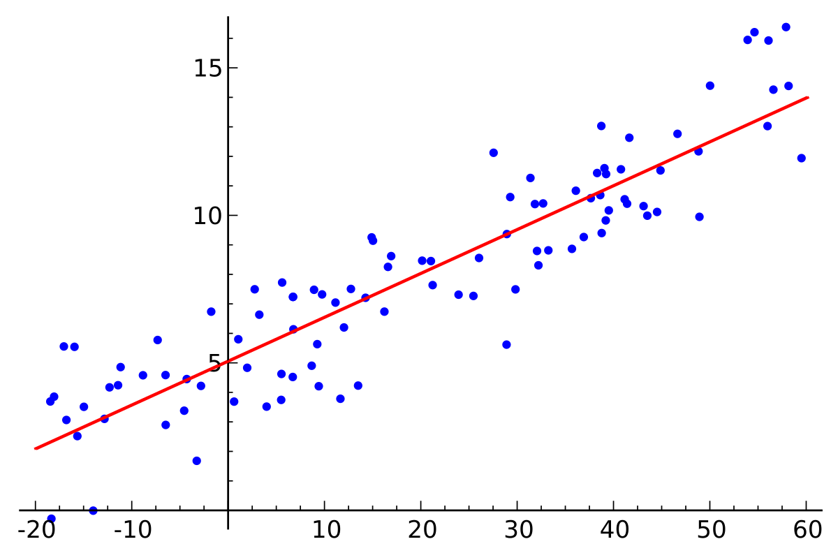
Linear Regression models the relationship between input (x) and output (y) as a straight line. It tries to minimize the difference between the predicted and actual values.
Example Diagram:
Python Code Example:
from sklearn.linear_model import LinearRegression
import numpy as np

# Sample data
X = np.array([[1], [2], [3], [4], [5]])
y = np.array([2, 4, 5, 4, 5])

# Create and train model
model = LinearRegression()
model.fit(X, y)

# Predict new values
y_pred = model.predict(np.array([[6]]))
print(f"Prediction for X=6: {y_pred[0]}")
2. Logistic Regression
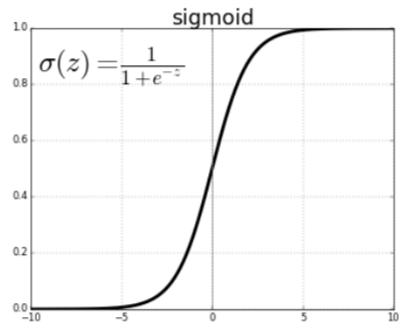
Logistic Regression is used for binary classification, predicting probabilities that the input belongs to one of two classes (e.g., "yes" or "no").
Example Diagram:
Python Code Example:
from sklearn.linear_model import LogisticRegression

# Sample data (1 or 0 outcome)
X = np.array([[1], [2], [3], [4], [5]])
y = np.array([0, 0, 0, 1, 1])

# Create and train model
model = LogisticRegression()
model.fit(X, y)

# Predict new value
y_pred = model.predict(np.array([[3.5]]))
print(f"Prediction for X=3.5: {y_pred[0]}")
3. Decision Tree Regression
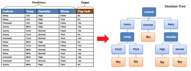
Decision Tree Regression splits the data into different regions based on decisions and forms a tree structure. Each leaf node represents a prediction.
Example Diagram:
Python Code Example:
from sklearn.tree import DecisionTreeRegressor

# Sample data
X = np.array([[1], [2], [3], [4], [5]])
y = np.array([1.5, 2.5, 3.0, 3.5, 4.0])

# Create and train model
model = DecisionTreeRegressor()
model.fit(X, y)

# Predict new values
y_pred = model.predict(np.array([[6]]))
print(f"Prediction for X=6: {y_pred[0]}")
4. Random Forest Regression
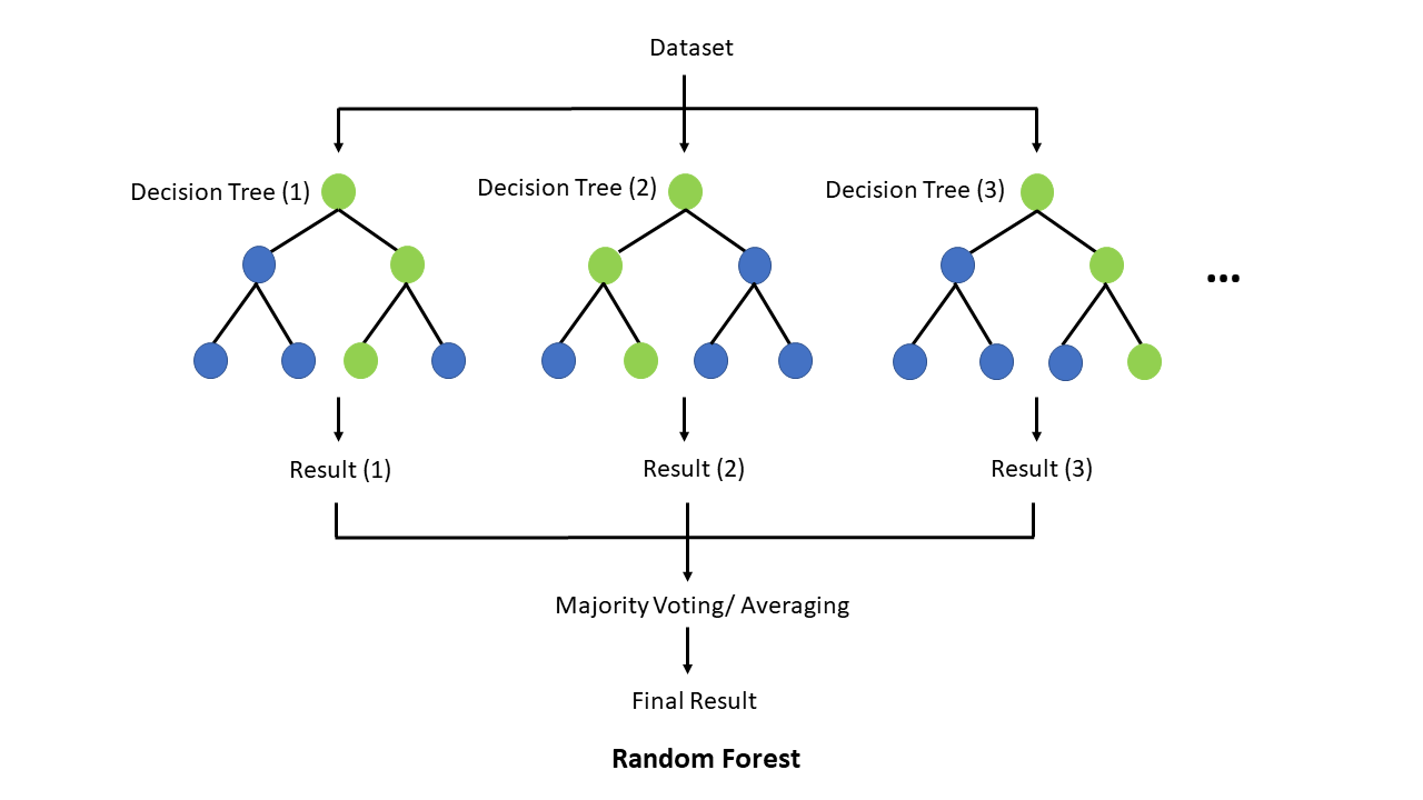
Random Forest Regression is an ensemble of multiple decision trees that makes predictions by averaging the results of the trees.
Example Diagram:
Python Code Example:
from sklearn.ensemble import RandomForestRegressor

# Sample data
X = np.array([[1], [2], [3], [4], [5]])
y = np.array([2, 4, 6, 8, 10])

# Create and train model
model = RandomForestRegressor(n_estimators=100)
model.fit(X, y)

# Predict new value
y_pred = model.predict(np.array([[6]]))
print(f"Prediction for X=6: {y_pred[0]}")
5. Support Vector Regression (SVR)
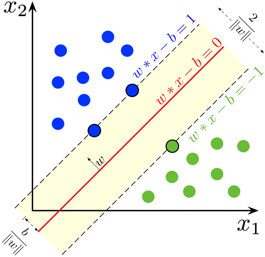
Support Vector Regression (SVR) fits the best line within a margin of error, known as the epsilon tube, focusing on points within this margin.
Example Diagram:
Python Code Example:
from sklearn.svm import SVR

# Sample data
X = np.array([[1], [2], [3], [4], [5]])
y = np.array([1, 2, 3, 5, 8])

# Create and train model
model = SVR(kernel='linear')
model.fit(X, y)

# Predict new value
y_pred = model.predict(np.array([[6]]))
print(f"Prediction for X=6: {y_pred[0]}")
6. K-Nearest Neighbors (KNN) Regression
KNN Regression finds the k-nearest data points to the input and predicts the value based on their average.
Example Diagram:

Python Code Example:
from sklearn.neighbors import KNeighborsRegressor

# Sample data
X = np.array([[1], [2], [3], [4], [5]])
y = np.array([1, 2, 1.5, 3.5, 2])

# Create and train model
model = KNeighborsRegressor(n_neighbors=2)
model.fit(X, y)

# Predict new value
y_pred = model.predict(np.array([[6]]))
print(f"Prediction for X=6: {y_pred[0]}")
7. Bayesian Linear Regression
Bayesian Linear Regression adds probability to the linear regression model, providing a measure of uncertainty in predictions.
Python Code Example:
from sklearn.linear_model import BayesianRidge

# Sample data
X = np.array([[1], [2], [3], [4], [5]])
y = np.array([1.2, 2.3, 3.1, 4.8, 5.5])

# Create and train model
model = BayesianRidge()
model.fit(X, y)

# Predict new value
y_pred = model.predict(np.array([[6]]))
print(f"Prediction for X=6: {y_pred[0]}")
8. Lasso and Ridge Regression
Lasso Regression and Ridge Regression add regularization to reduce overfitting in linear regression. Lasso uses L1 regularization (shrinking coefficients to zero), while Ridge uses L2 regularization.
Lasso Regression Code Example:
from sklearn.linear_model import Lasso

# Sample data
X = np.array([[1], [2], [3], [4], [5]])
y = np.array([2, 3, 4, 5, 6])

# Create and train model
model = Lasso(alpha=0.1)
model.fit(X, y)

# Predict new value
y_pred = model.predict(np.array([[6]]))
print(f"Prediction for X=6: {y_pred[0]}")
Ridge Regression Code Example:
from sklearn.linear_model import Ridge

# Create and train model
model = Ridge(alpha=1.0)
model.fit(X, y)

# Predict new value
y_pred = model.predict(np.array([[6]]))
print(f"Prediction for X=6: {y_pred[0]}")
9. Regression Analysis
Regression Analysis helps understand the relationships between variables, often used in fields such as economics and biology.
10. Neural Networks with Regression
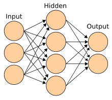
Neural Networks can capture complex relationships between variables. For regression, the output layer of the network predicts continuous values.
Example Diagram:
Python Code Example (Using Keras):
from tensorflow.keras.models import Sequential
from tensorflow.keras.layers import Dense

# Sample data
X = np.array([[1], [2], [3], [4], [5]])
y = np.array([1, 2, 3, 4, 5])

# Create neural network model
model = Sequential()
model.add(Dense(10, input_dim=1, activation='relu'))
model.add(Dense(1))  # Output layer

# Compile and train model
model.compile(optimizer='adam', loss='mean_squared_error')
model.fit(X, y, epochs=100, verbose=0)

# Predict new value
y_pred = model.predict(np

.array([[6]]))
print(f"Prediction for X=6: {y_pred[0][0]}")
Conclusion
Each regression algorithm has its strengths and is suited for different tasks. Linear regression works well for simple data, while Random Forests and Neural Networks are ideal for more complex datasets. Learning and experimenting with these algorithms will help you solve a variety of predictive problems.