3 posts tagged with "llm"

View All Tags

Inside the WhereQ Universe: One Identity, Many Apps, Open APIs

· 7 min read

The WhereQ Universe is not a single product — it is a living ecosystem of independent applications that share one identity layer, one set of engineering conventions, and an increasingly open set of APIs. This post walks through how the pieces fit together: why authentication lives in a single place, how the apps expose data to customers, and where LLM agents and MCP fit into the picture.

Full Fine-Tuning vs LoRA

· 21 min read

Table of Contents​

  1. Introduction
  2. What is Fine-Tuning?
  3. Full Fine-Tuning Explained
  4. LoRA (Low-Rank Adaptation) Explained
  5. Technical Comparison
  6. Real-World Use Cases
  7. When to Use Which Method
  8. Hands-On Practice Guide
  9. Advanced Topics
  10. Decision Framework

Introduction​

In the era of Large Language Models (LLMs), fine-tuning has become the key to adapting pre-trained models to specific tasks. Two main approaches dominate the landscape:

  • Full Fine-Tuning: Training all model parameters
  • LoRA (Low-Rank Adaptation): Training only a small subset of parameters

What is Fine-Tuning?​

Simple Analogy​

Think of a pre-trained model as a medical doctor with general knowledge. Fine-tuning is like:

  • Full Fine-Tuning: Sending the doctor back to medical school to relearn everything with a focus on a specialty
  • LoRA: Giving the doctor a specialized handbook they can reference without forgetting their general knowledge

Technical Definition​

Fine-tuning takes a pre-trained model (trained on massive general data) and continues training it on domain-specific data to improve performance on particular tasks.

Pre-trained Model (General Knowledge)
↓
Fine-Tuning (Specialized Training)
↓
Task-Specific Model (Expert Knowledge)

Full Fine-Tuning Explained​

What is Full Fine-Tuning?​

Full fine-tuning means updating ALL parameters in the model during training.

Model Architecture (Example: 7B parameters)
┌──────────────────────────────────────┐
│ Layer 1: [All parameters trainable] │ ← Updated
│ Layer 2: [All parameters trainable] │ ← Updated
│ Layer 3: [All parameters trainable] │ ← Updated
│ ... │ ← Updated
│ Layer N: [All parameters trainable] │ ← Updated
└──────────────────────────────────────┘
Total Trainable: 7,000,000,000 params

How It Works​

  1. Load pre-trained model (e.g., GPT-3, LLaMA, ChatGLM)
  2. Prepare task-specific dataset (e.g., medical Q&A, legal documents)
  3. Train ALL parameters using your dataset
  4. Save the entire model (full 7B+ parameters)

Advantages ✅​

  1. Maximum Performance: Can achieve the best possible results
  2. Deep Customization: All parameters adapt to your specific task
  3. Flexible: Works for any task, especially those very different from pre-training

Disadvantages ❌​

  1. Extremely High Cost:

    • GPT-3 175B full fine-tuning requires >2TB GPU memory
    • Needs high-end GPU clusters (multiple A100s)
    • Training can cost $20,000+ per run
  2. Long Training Time: Days or weeks to complete

  3. Storage Overhead:

    • Each task needs a complete model copy
    • 7B model = ~14GB storage per task
    • 10 tasks = 140GB storage needed
  4. Catastrophic Forgetting:

    • Model may lose general knowledge
    • Reduced generalization ability

Real-World Example​

Google's Multilingual Search Optimization

  • Used full fine-tuning on BERT-Large for multilingual search
  • Result: 25% improvement in low-resource language recall
  • Cost: Requires massive GPU infrastructure
  • Benefit: State-of-the-art performance across 100+ languages

LoRA (Low-Rank Adaptation) Explained​

What is LoRA?​

LoRA is a parameter-efficient fine-tuning method proposed by Microsoft in 2021. Instead of updating all parameters, LoRA:

  • Freezes the original model weights
  • Adds small "adapter" matrices to specific layers
  • Trains only these tiny adapters (typically 0.1%-1% of total parameters)

Visual Explanation​

Original Transformer Layer
┌────────────────────────────────────────┐
│ Pre-trained Weight Matrix W │
│ [Frozen - Not Updated] │
│ + │
│ Low-Rank Adapter: A × B │
│ [Trainable - Only These Updated] │
└────────────────────────────────────────┘

Output = W·x + A·B·x
↑ ↑
Frozen Trained (tiny!)

Mathematical Foundation​

For a pre-trained weight matrix W (dimension d × k):

Full Fine-Tuning:
Updates: ΔW (d × k parameters)
Total trainable: d × k

LoRA:
Decomposes: ΔW ≈ A × B
Where: A is (d × r), B is (r × k)
Total trainable: d×r + r×k

Example (d=4096, k=4096, r=8):
Full: 4096 × 4096 = 16,777,216 params
LoRA: 4096×8 + 8×4096 = 65,536 params
Reduction: 99.6%! 🎉

How LoRA Works (Step-by-Step)​

  1. Freeze Original Model

    for param in pretrained_model.parameters():
    param.requires_grad = False # Don't update these
  2. Inject Low-Rank Matrices

    • Insert matrices A and B into attention layers
    • Initialize: A with random values, B with zeros
    • Typically apply to Query, Value projection matrices
  3. Train Only Adapters

    for param in lora_adapters.parameters():
    param.requires_grad = True # Only update these
  4. Inference

    output = original_weight @ x + (A @ B) @ x

Advantages ✅​

  1. Extreme Parameter Efficiency:

    • Reduces trainable parameters by 90-99%
    • 7B model: Train only 7-70M parameters instead of 7B
  2. Low Cost, Fast Deployment:

    • Consumer GPU (RTX 4090, RTX 3090) can fine-tune large models
    • Training time: Hours instead of days
    • Cost: **50−200∗∗insteadof50-200** instead of 20,000+
  3. Multi-Task Flexibility:

    • Save only adapter weights (~10-100MB per task)
    • Dynamically load different adapters for different tasks
    • One base model + multiple adapters = multiple specialized models
  4. Less Catastrophic Forgetting:

    • Original weights unchanged
    • Retains general knowledge better

Disadvantages ❌​

  1. Rank Parameter Tuning Required:

    • Too small r (rank) → underfitting
    • Too large r → loses efficiency
    • Needs experimentation
  2. "Intruder Dimensions" Problem (Recent Discovery):

    • LoRA introduces high-ranking singular vectors
    • Reduces out-of-distribution (OOD) generalization by 5-8%
    • Less robust in continual learning scenarios
  3. Slightly Lower Peak Performance:

    • May not reach absolute best performance
    • Gap is usually small (<1-3%) for most tasks

Real-World Examples​

1. Medical Document Summarization

  • Hospital used LoRA to fine-tune GPT-3 for medical report generation
  • Result: High-quality summaries, doctor efficiency increased 40%
  • Cost: Single RTX A6000 GPU, trained in 6 hours
  • Storage: Base model (14GB) + Adapter (50MB)

2. E-commerce Customer Service

  • Online retailer fine-tuned ChatGLM for customer support
  • Result: Response speed improved 3x, satisfaction up 25%
  • Deployment: 5 different product category adapters
  • Total storage: One model + 5 adapters = 14.3GB (vs 70GB for 5 full models)

3. Financial News Generation

  • News agency fine-tuned GPT-3 for real-time financial reporting
  • Result: News generation latency reduced to seconds, 40% cost reduction
  • Adaptation time: 4 hours on 2× RTX 4090

Technical Comparison​

Architecture Comparison​

FULL FINE-TUNING
════════════════════════════════════════
Input → [Layer 1 ✏️] → [Layer 2 ✏️] → [Layer 3 ✏️] → Output
All Updated All Updated All Updated

LoRA
════════════════════════════════════════
Input → [Layer 1 🔒] → [Layer 2 🔒] → [Layer 3 🔒] → Output
+ Adapter✏️ + Adapter✏️ + Adapter✏️

🔒 = Frozen (unchanged)
✏️ = Trainable (updated during training)

Detailed Comparison Table​

AspectFull Fine-TuningLoRA
Trainable Parameters100% (e.g., 7B params)0.1-1% (e.g., 7-70M params)
GPU MemoryVery High (>80GB for 7B)Low (24-48GB for 7B)
Training TimeDays to weeksHours to 1-2 days
Cost per Training10,000−10,000 - 100,000+50−50 - 500
Storage per TaskFull model (~14GB for 7B)Adapter only (~10-100MB)
PerformanceHighest (100% baseline)Very High (95-99% of full)
Multi-Task DeploymentDifficult (one model per task)Easy (one model + N adapters)
Catastrophic ForgettingHigh riskLow risk
Hardware RequirementsHigh-end GPU cluster (A100×8)Consumer GPU (RTX 3090/4090)
Generalization (OOD)BestGood (5-8% lower)
Best ForMaximum performance, unlimited budgetFast iteration, limited resources

Memory Comparison (7B Model Example)​

Full Fine-Tuning (7B parameters):
┌─────────────────────────────────┐
│ Model: 14GB │
│ Optimizer States: 42GB │
│ Gradients: 14GB │
│ Activations: 20GB │
│ ─────────────────────────────── │
│ Total: ~90GB │
└─────────────────────────────────┘
Required: 4× A100 (40GB each)

LoRA (7B base + 10M adapter):
┌─────────────────────────────────┐
│ Base Model: 14GB (frozen) │
│ Adapter: 20MB │
│ Optimizer States: 60MB │
│ Gradients: 20MB │
│ Activations: 12GB │
│ ─────────────────────────────── │
│ Total: ~27GB │
└─────────────────────────────────┘
Required: 1× RTX 3090/4090 (24GB)

Real-World Use Cases​

Use Case 1: Healthcare - Clinical Note Generation​

Scenario: Hospital needs AI to generate structured clinical notes from doctor-patient conversations.

Challenge:

  • Medical terminology requires domain adaptation
  • HIPAA compliance = can't use cloud APIs
  • Limited budget and GPU resources

Solution: LoRA Fine-Tuning

# Approach
Base Model: LLaMA-2-7B
Dataset: 10,000 anonymized clinical conversations
Training: LoRA (r=16, α=32)
Hardware: 1× RTX A6000 (48GB)
Time: 8 hours
Cost: ~$100

# Results
- Accuracy: 94% (vs 96% with full fine-tuning)
- Deployment: One base model + adapter (14.05GB total)
- Multi-specialty: 5 adapters for different departments (14.3GB total)

Why LoRA Won:

  • ✅ Budget-friendly
  • ✅ Fast iteration for different specialties
  • ✅ Meets accuracy requirements
  • ✅ Easy deployment on-premise

Scenario: Law firm needs to analyze merger & acquisition contracts for risk factors.

Challenge:

  • Complex legal language
  • High accuracy requirement (mistakes = legal liability)
  • Contracts vary significantly by jurisdiction

Solution: Full Fine-Tuning

# Approach
Base Model: GPT-3.5-turbo-instruct
Dataset: 50,000 labeled M&A contracts
Training: Full fine-tuning all parameters
Hardware: 8× A100 GPUs (cloud)
Time: 4 days
Cost: ~$25,000

# Results
- Accuracy: 98.5% (vs 95% with LoRA r=64)
- Risk detection: 99.2% recall (critical for legal)
- False positive rate: 1.8% (vs 4.2% with LoRA)

Why Full Fine-Tuning Won:

  • ✅ Maximum accuracy needed (legal liability)
  • ✅ Budget available (law firm can afford)
  • ✅ Single specialized task
  • ✅ 3% accuracy improvement = millions in risk mitigation

Use Case 3: E-Commerce - Multi-Category Product Descriptions​

Scenario: Online marketplace needs to generate product descriptions for 10 different categories (electronics, fashion, home, etc.).

Challenge:

  • 10 different writing styles needed
  • Rapid product launches (new categories added quarterly)
  • Budget-conscious startup

Solution: LoRA with Multi-Adapter Architecture

# Approach
Base Model: Qwen-7B
Training: 10 separate LoRA adapters (r=8)
- Electronics adapter
- Fashion adapter
- Home & Garden adapter
- Sports adapter
- ... (6 more)
Hardware: 1× RTX 4090
Time per adapter: 3 hours
Total cost: ~$300

# Deployment
Storage:
Base model: 14GB
10 adapters: 10 × 40MB = 400MB
Total: 14.4GB (vs 140GB for 10 full models)

# Runtime
Load base model once, swap adapters dynamically:
electronics_model = base + electronics_adapter
fashion_model = base + fashion_adapter

Why LoRA Won:

  • ✅ 10× storage savings
  • ✅ Can train new category adapter in hours
  • ✅ Single GPU deployment
  • ✅ Easy A/B testing different adapters

Use Case 4: Multilingual Customer Support​

Scenario: Global SaaS company needs chatbots for 20 languages.

Challenge:

  • 20 language-specific models needed
  • Need to update all models when features change
  • Some languages low-resource (limited training data)

LoRA Approach (Recommended):

Base Model: Multilingual LLaMA-2-13B
Training: 20 language adapters (r=16)

Storage: 26GB base + (20 × 80MB) = 27.6GB
vs Full Fine-Tuning: 20 × 26GB = 520GB

Benefit: Update base model → all languages benefit

When to Use Which Method​

Choose Full Fine-Tuning When:​

  1. Maximum Performance is Critical ✅

    • Legal, medical, financial applications where errors are costly
    • Need that extra 2-5% accuracy
  2. Large Dataset Available ✅

    • Have >100,000 high-quality labeled examples
    • Data justifies training all parameters
  3. Unlimited Budget & Resources ✅

    • Access to GPU clusters (8+ A100s)
    • Can afford $10,000-100,000 training costs
  4. Single Specialized Task ✅

    • Only need one model for one task
    • No plan for multi-task deployment
  5. Task Very Different from Pre-training ✅

    • Specialized domains (medical, legal, scientific)
    • Low-resource languages

Example Decision:

Use Full Fine-Tuning if:
(Accuracy_requirement > 97%) AND
(Budget > $10,000) AND
(Single_task OR Task_very_different)

Choose LoRA When:​

  1. Limited Resources ✅

    • Budget < $5,000
    • Only have consumer GPUs (RTX 3090, 4090)
  2. Need Fast Iteration ✅

    • Startup environment
    • Frequent model updates
    • Rapid experimentation
  3. Multi-Task Deployment ✅

    • Need models for 5+ different tasks/domains
    • Want to switch between tasks dynamically
  4. Storage Constraints ✅

    • Limited disk space
    • Edge device deployment
  5. Continuous Learning ✅

    • Need to add new capabilities over time
    • Can't afford catastrophic forgetting

Example Decision:

Use LoRA if:
(Budget < $5,000) OR
(GPU_memory < 80GB) OR
(Num_tasks > 3) OR
(Need_fast_iteration)

Hands-On Practice Guide​

Prerequisites​

# Install required libraries
pip install torch transformers peft datasets accelerate bitsandbytes

# Check GPU
nvidia-smi

Practice 1: Full Fine-Tuning (Small Model)​

Task: Fine-tune GPT-2 (small) for custom text generation

from transformers import GPT2LMHeadModel, GPT2Tokenizer, Trainer, TrainingArguments
from datasets import load_dataset

# 1. Load pre-trained model
model = GPT2LMHeadModel.from_pretrained("gpt2")
tokenizer = GPT2Tokenizer.from_pretrained("gpt2")
tokenizer.pad_token = tokenizer.eos_token

# 2. Prepare dataset
dataset = load_dataset("wikitext", "wikitext-2-raw-v1")

def tokenize_function(examples):
return tokenizer(examples["text"], truncation=True,
max_length=512, padding="max_length")

tokenized_datasets = dataset.map(tokenize_function, batched=True)

# 3. Training configuration (FULL FINE-TUNING)
training_args = TrainingArguments(
output_dir="./gpt2-finetuned-full",
num_train_epochs=3,
per_device_train_batch_size=4,
save_steps=500,
save_total_limit=2,
learning_rate=2e-5,
# All parameters trainable (default)
)

# 4. Train
trainer = Trainer(
model=model,
args=training_args,
train_dataset=tokenized_datasets["train"],
)

trainer.train()

# 5. Save model
model.save_pretrained("./gpt2-finetuned-full")
tokenizer.save_pretrained("./gpt2-finetuned-full")

print(f"Model size: {sum(p.numel() for p in model.parameters())} parameters")
# Output: ~124M parameters all trained

Resource Requirements:

  • GPU: GTX 1080 Ti or better (11GB+)
  • Time: ~2 hours
  • Storage: ~500MB

Practice 2: LoRA Fine-Tuning (Large Model)​

Task: Fine-tune LLaMA-2-7B for instruction following using LoRA

from transformers import AutoModelForCausalLM, AutoTokenizer, TrainingArguments
from peft import LoraConfig, get_peft_model, prepare_model_for_kbit_training
from datasets import load_dataset
from trl import SFTTrainer

# 1. Load base model (with 4-bit quantization for efficiency)
model_name = "meta-llama/Llama-2-7b-hf"
model = AutoModelForCausalLM.from_pretrained(
model_name,
load_in_4bit=True, # Quantization to reduce memory
device_map="auto"
)
tokenizer = AutoTokenizer.from_pretrained(model_name)
tokenizer.pad_token = tokenizer.eos_token

# 2. Configure LoRA
lora_config = LoraConfig(
r=16, # Rank (try 8, 16, 32, 64)
lora_alpha=32, # Scaling factor
target_modules=["q_proj", "v_proj"], # Apply to attention
lora_dropout=0.05,
bias="none",
task_type="CAUSAL_LM"
)

# 3. Prepare model for LoRA training
model = prepare_model_for_kbit_training(model)
model = get_peft_model(model, lora_config)

# Print trainable parameters
model.print_trainable_parameters()
# Output: trainable params: 4,194,304 || all params: 6,738,415,616 || trainable%: 0.06%

# 4. Load instruction dataset
dataset = load_dataset("timdettmers/openassistant-guanaco")

# 5. Training configuration
training_args = TrainingArguments(
output_dir="./llama2-lora",
num_train_epochs=3,
per_device_train_batch_size=4,
gradient_accumulation_steps=4,
learning_rate=2e-4,
logging_steps=10,
save_strategy="epoch",
fp16=True, # Mixed precision
)

# 6. Train with SFTTrainer (Supervised Fine-Tuning)
trainer = SFTTrainer(
model=model,
train_dataset=dataset["train"],
args=training_args,
peft_config=lora_config,
dataset_text_field="text",
max_seq_length=512,
)

trainer.train()

# 7. Save only LoRA adapter (tiny!)
model.save_pretrained("./llama2-lora-adapter")

# 8. Load and use later
from peft import PeftModel

base_model = AutoModelForCausalLM.from_pretrained(model_name)
lora_model = PeftModel.from_pretrained(base_model, "./llama2-lora-adapter")

# Generate
inputs = tokenizer("Explain quantum computing:", return_tensors="pt")
outputs = lora_model.generate(**inputs, max_length=100)
print(tokenizer.decode(outputs[0]))

Resource Requirements:

  • GPU: RTX 3090 (24GB) or better
  • Time: 4-8 hours
  • Storage: Base model (14GB) + Adapter (50MB)

Key Observations:

  • Only 0.06% of parameters trained! (4M out of 6.7B)
  • Memory usage: ~18GB (vs ~90GB for full fine-tuning)
  • Can train multiple adapters and switch between them

Practice 3: Comparing LoRA Ranks​

Experiment: Train same model with different ranks and compare

# Train adapters with different ranks
ranks = [4, 8, 16, 32, 64]
results = {}

for r in ranks:
print(f"\n{'='*50}")
print(f"Training with rank r={r}")
print(f"{'='*50}")

lora_config = LoraConfig(
r=r,
lora_alpha=r*2, # Common practice: alpha = 2*r
target_modules=["q_proj", "v_proj"],
lora_dropout=0.05,
bias="none",
task_type="CAUSAL_LM"
)

model = prepare_model_for_kbit_training(base_model)
model = get_peft_model(model, lora_config)

# Train and evaluate
trainer = SFTTrainer(...)
trainer.train()
metrics = trainer.evaluate()

results[r] = {
'trainable_params': sum(p.numel() for p in model.parameters() if p.requires_grad),
'loss': metrics['eval_loss'],
'adapter_size_mb': get_adapter_size(model)
}

# Compare results
import pandas as pd
df = pd.DataFrame(results).T
print(df)

# Expected output:
# trainable_params loss adapter_size_mb
# 4 2,097,152 2.45 8
# 8 4,194,304 2.31 16
# 16 8,388,608 2.24 32
# 32 16,777,216 2.21 64
# 64 33,554,432 2.19 128

Insights:

  • Rank 4-8: Fast, tiny, good for simple tasks
  • Rank 16-32: Sweet spot for most tasks
  • Rank 64+: Approaching full fine-tuning performance

Advanced Topics​

1. QLoRA (Quantized LoRA)​

What: Combines LoRA with 4-bit quantization for even lower memory usage.

Breakthrough: Train 65B parameter models on a single 48GB GPU!

from transformers import BitsAndBytesConfig

# QLoRA configuration
bnb_config = BitsAndBytesConfig(
load_in_4bit=True,
bnb_4bit_use_double_quant=True,
bnb_4bit_quant_type="nf4",
bnb_4bit_compute_dtype=torch.bfloat16
)

model = AutoModelForCausalLM.from_pretrained(
"meta-llama/Llama-2-70b-hf",
quantization_config=bnb_config,
device_map="auto"
)

# Now train with LoRA as before
# Memory usage: ~40GB for 70B model! 🎉

Use Case: Fine-tune massive models (65B, 70B+) on consumer hardware.


2. AdaLoRA (Adaptive LoRA)​

What: Dynamically adjusts rank during training based on importance.

Benefit: Automatically finds optimal rank per layer.

from peft import AdaLoraConfig, get_peft_model

adalora_config = AdaLoraConfig(
init_r=12, # Initial rank
target_r=8, # Target rank
tinit=200, # Warmup steps
tfinal=1000, # Total steps
delta_t=10, # Rank adjustment frequency
beta1=0.85,
beta2=0.85,
orth_reg_weight=0.5,
lora_alpha=32,
lora_dropout=0.1,
target_modules=["q_proj", "v_proj"],
task_type="CAUSAL_LM"
)

model = get_peft_model(model, adalora_config)

Result: Better performance than fixed-rank LoRA with similar parameter count.


3. The "Intruder Dimensions" Problem​

Recent Discovery (MIT Research, 2024):

LoRA introduces high-ranking singular vectors not present in full fine-tuning. These "intruder dimensions":

  • Reduce out-of-distribution generalization by 5-8%
  • Cause more forgetting in continual learning
  • Appear more with lower ranks (r ≤ 16)

Visualization:

Full Fine-Tuning Weight Matrix SVD:
Singular Values: [100, 95, 90, 85, 80, ...] ← Smooth decay
Singular Vectors: All similar to pre-trained

LoRA Weight Matrix SVD:
Singular Values: [100, 95, 90, 85, 80, ..., 15, 14, 13] ← Similar
↓
[50, 45, 40] ← INTRUDER!
Singular Vectors: Some very different from pre-trained

Solutions:

  1. Use higher rank (r=64+) with rank stabilization
  2. Use "rank-stabilized LoRA" techniques
  3. For critical applications, prefer full fine-tuning

4. Multi-Adapter Architecture​

Pattern: One base model + dynamic adapter loading

# Training phase: Train multiple adapters
adapters = {
'medical': train_lora(base_model, medical_data, r=16),
'legal': train_lora(base_model, legal_data, r=16),
'finance': train_lora(base_model, finance_data, r=16),
}

# Save adapters
for name, adapter in adapters.items():
adapter.save_pretrained(f"./adapters/{name}")

# Inference phase: Dynamically load adapters
from peft import PeftModel

base_model = AutoModelForCausalLM.from_pretrained("llama-2-7b")

# For medical query
medical_model = PeftModel.from_pretrained(base_model, "./adapters/medical")
response = medical_model.generate(...)

# Switch to legal
legal_model = PeftModel.from_pretrained(base_model, "./adapters/legal")
response = legal_model.generate(...)

# Or merge multiple adapters!
from peft import PeftModel
multi_model = PeftModel.from_pretrained(base_model, "./adapters/medical")
multi_model.load_adapter("./adapters/legal", adapter_name="legal")
multi_model.set_adapter(["medical", "legal"]) # Use both!

Decision Framework​

The Complete Decision Tree​

START: Do you need to fine-tune a large language model?
│
├─→ Q1: What's your budget?
│ ├─→ < $1,000: → LoRA (or QLoRA)
│ ├─→ $1,000 - $10,000: → LoRA (consider full if single critical task)
│ └─→ > $10,000: → Consider full fine-tuning
│
├─→ Q2: What GPU do you have?
│ ├─→ Consumer (RTX 3090/4090): → LoRA or QLoRA
│ ├─→ Single A100 (40-80GB): → LoRA or Full (for <7B models)
│ └─→ GPU Cluster (8+ A100s): → Full fine-tuning possible
│
├─→ Q3: How many tasks?
│ ├─→ 1 task: → Either (depends on other factors)
│ ├─→ 2-5 tasks: → LoRA (multi-adapter)
│ └─→ 5+ tasks: → Definitely LoRA
│
├─→ Q4: Accuracy requirements?
│ ├─→ >98% required: → Full fine-tuning
│ ├─→ 95-98%: → LoRA (high rank, r=64+)
│ └─→ <95%: → LoRA (standard rank, r=8-16)
│
├─→ Q5: Deployment constraints?
│ ├─→ Edge devices: → LoRA (smaller)
│ ├─→ Cloud: → Either
│ └─→ Need rapid updates: → LoRA
│
└─→ Q6: Continual learning needed?
├─→ Yes, multiple sequential tasks: → High-rank LoRA or Full
├─→ No: → Standard LoRA
└─→ Critical to avoid forgetting: → Full fine-tuning

Quick Selection Matrix​

Your SituationRecommended MethodRank/Config
Startup, limited GPU, 3+ tasksLoRAr=8-16
Enterprise, single critical taskFull Fine-TuningAll parameters
Research, multiple experimentsLoRAr=16-32
>100B model, limited hardwareQLoRAr=8-16, 4-bit
Medical/Legal high-stakesFull Fine-TuningAll parameters
Multi-lingual deploymentLoRA multi-adapterr=16 per language
Rapid A/B testingLoRAr=8 (fast training)
Edge device deploymentQLoRAr=4-8, quantized

Best Practices & Tips​

For LoRA Fine-Tuning​

  1. Start Small, Scale Up

    # Experiment progression
    1. Try r=8 first (fast, good baseline)
    2. If underfitting, increase to r=16
    3. For complex tasks, try r=32 or r=64
    4. Monitor validation loss to find sweet spot
  2. Target the Right Modules

    # For most language models
    target_modules = ["q_proj", "v_proj"] # Minimum (queries & values)

    # For better performance
    target_modules = ["q_proj", "k_proj", "v_proj", "o_proj"] # All attention

    # For maximum adaptation (more params)
    target_modules = ["q_proj", "k_proj", "v_proj", "o_proj",
    "gate_proj", "up_proj", "down_proj"] # Attention + FFN
  3. Learning Rate Selection

    # LoRA typically needs higher LR than full fine-tuning
    Full Fine-Tuning: lr = 1e-5 to 5e-5
    LoRA: lr = 1e-4 to 3e-4 (10x higher!)

    # Rule of thumb
    lora_lr = full_finetuning_lr * 10
  4. Rank Selection Guide

    Task Complexity → Recommended Rank
    ─────────────────────────────────────────
    Simple (sentiment) → r=4-8
    Medium (summarization) → r=8-16
    Complex (reasoning) → r=16-32
    Very complex (coding) → r=32-64
    Approaching full FT → r=128-256
  5. Prevent Intruder Dimensions

    # Use rank stabilization
    lora_config = LoraConfig(
    r=32,
    lora_alpha=64,
    use_rslora=True, # Rank-stabilized LoRA
    # ... other params
    )

For Full Fine-Tuning​

  1. Gradient Checkpointing (Save Memory)

    model.gradient_checkpointing_enable()
    # Trades computation for memory
    # Enables training larger models on same GPU
  2. Mixed Precision Training

    training_args = TrainingArguments(
    fp16=True, # For older GPUs
    bf16=True, # For A100s (better for large models)
    # Reduces memory usage by 2x
    )
  3. Distributed Training

    # Use DeepSpeed for multi-GPU
    training_args = TrainingArguments(
    deepspeed="ds_config.json",
    per_device_train_batch_size=1,
    gradient_accumulation_steps=16,
    )

    # ds_config.json
    {
    "train_batch_size": "auto",
    "zero_optimization": {
    "stage": 3, # ZeRO-3: Shard everything
    }
    }
  4. Prevent Catastrophic Forgetting

    # Use lower learning rate
    learning_rate = 1e-5 # vs 2e-4 for pre-training

    # Freeze some layers (partial fine-tuning)
    for i, layer in enumerate(model.layers):
    if i < 20: # Freeze first 20 layers
    for param in layer.parameters():
    param.requires_grad = False

    # Use elastic weight consolidation (EWC)
    # Add regularization term penalizing large weight changes

Common Mistakes & How to Avoid Them​

Mistake 1: Using LoRA rank that's too low​

❌ Problem: r=4 for complex instruction following

lora_config = LoraConfig(r=4, ...) # Too small!
# Result: Model can't learn complex patterns, poor performance

✅ Solution: Start with r=16, increase if needed

lora_config = LoraConfig(r=16, lora_alpha=32, ...)
# Monitor validation loss, increase to r=32 if plateauing

Mistake 2: Wrong learning rate​

❌ Problem: Using same LR for LoRA as full fine-tuning

# Full fine-tuning LR used for LoRA
training_args = TrainingArguments(learning_rate=2e-5, ...)
# Result: Slow convergence, underfitting

✅ Solution: Use 10x higher LR for LoRA

training_args = TrainingArguments(learning_rate=2e-4, ...)
# LoRA adapters need stronger signals to learn

Mistake 3: Not quantizing when memory is tight​

❌ Problem: Trying to load 7B model in FP16 on 16GB GPU

model = AutoModelForCausalLM.from_pretrained("llama-2-7b")
# Result: CUDA Out of Memory error

✅ Solution: Use 4-bit/8-bit quantization

model = AutoModelForCausalLM.from_pretrained(
"llama-2-7b",
load_in_4bit=True,
device_map="auto"
)
# Result: Fits in 8GB GPU!

Mistake 4: Training on too few examples​

❌ Problem: Fine-tuning on 100 examples

dataset = load_dataset(...)[:100] # Only 100 examples
# Result: Overfitting, poor generalization

✅ Solution: Minimum dataset sizes

Full Fine-Tuning: 10,000+ examples (ideally 100k+)
LoRA: 1,000+ examples (can work with 500 for simple tasks)
QLoRA: 500+ examples (most efficient)

If you have <500 examples:
→ Use prompt engineering or few-shot learning instead

Mistake 5: Not saving checkpoints​

❌ Problem: Training crashes after 20 hours, no checkpoints

training_args = TrainingArguments(
save_strategy="no", # Dangerous!
)

✅ Solution: Regular checkpointing

training_args = TrainingArguments(
save_strategy="steps",
save_steps=500,
save_total_limit=3, # Keep last 3 checkpoints
)

Real Cost Comparison​

Example: Fine-tuning LLaMA-2-7B for 3 epochs on 10,000 examples​

Full Fine-Tuning:

Hardware: 4× A100 (80GB) via AWS
Cost: $32.77/hour per GPU
Duration: 48 hours
Total: $32.77 × 4 × 48 = $6,293

Storage: 14GB per model
If 5 tasks: 70GB total

Total Investment: ~$6,300 + ongoing storage

LoRA (r=16):

Hardware: 1× RTX 4090 (24GB) - owned or $2/hour cloud
Cost: $2/hour
Duration: 12 hours
Total: $2 × 12 = $24

Storage: 14GB base + (5 × 50MB adapters) = 14.25GB

Total Investment: ~$24 + one-time GPU purchase (~$1,600)

Savings: 99.6% 🎉


1. LoRA+ and LoRA-FA​

  • LoRA+: Different learning rates for A and B matrices
  • LoRA-FA: Frozen-A variant (only train B matrix)
  • Result: Faster convergence, better performance

2. DoRA (Weight-Decomposed LoRA)​

  • Decomposes weights into magnitude and direction
  • Bridges gap between LoRA and full fine-tuning
  • 20% better performance on reasoning tasks

3. MultiLoRA & LoRA Composition​

  • Train multiple LoRA adapters
  • Compose them at inference time
  • Example: (medical_adapter × 0.7) + (general_adapter × 0.3)

4. LoRA for Vision & Multimodal Models​

  • VoRA: LoRA for vision transformers
  • Successful for CLIP, Stable Diffusion fine-tuning
  • 90% memory reduction for image model fine-tuning

Summary & Recommendations​

The Bottom Line​

LoRA is the default choice for most practitioners in 2024-2025.

Reasons:

  • ✅ 99% cost reduction
  • ✅ Accessible on consumer hardware
  • ✅ Fast iteration (hours vs days)
  • ✅ Easy multi-task deployment
  • ✅ Good enough performance for most applications (95-99% of full)

Full Fine-Tuning is for special cases:

  • High-stakes applications (medical, legal, financial)
  • Unlimited budget and resources
  • Need absolute best performance
  • Research settings exploring model limits

Your Action Plan​

Week 1: Start with LoRA

1. Choose base model (LLaMA-2-7B, Mistral-7B, Qwen)
2. Prepare 1,000+ examples
3. Train LoRA (r=16) on 1× GPU
4. Evaluate on validation set
5. Iterate on rank and hyperparameters

Week 2: Optimize

1. Experiment with ranks: 8, 16, 32
2. Try different target modules
3. Test QLoRA if memory constrained
4. A/B test different adapters

Month 2+: Scale if Needed

if performance < requirements:
if budget_available:
try full fine-tuning
else:
try higher rank LoRA (r=64-128)
or try DoRA/LoRA+ variants

Additional Resources​

Code Repositories​

Tutorials​

Communities​


Remember:

  • Start with LoRA (r=16)
  • Scale to full fine-tuning only if truly needed
  • Focus on data quality over method choice
  • Iterate quickly and measure results

The best method is the one that:

  1. Fits your budget
  2. Meets your accuracy requirements
  3. Enables fast iteration
  4. Scales with your needs

Plain Language Explanation of Large Models

· 21 min read

Introduction​

This document aims to provide a detailed explanation of the current mainstream large model architectures, such as the Transformer architecture. We will cover various aspects from a technical overview, architecture introduction to specific model implementations. Through this document, we hope to provide readers with a comprehensive understanding, helping them grasp the working principles of large models and enhance their technical foundation for communicating with clients. This document is suitable for individuals interested in large models.

Paper Introduction​

Paper Title: Attention is all you need

Release Date: 2017/06/12

Published By: Google, University of Toronto

Brief Summary: The progenitor of all LLMs, the foundational architecture for a new era in NLP.

Chinese Summary: Traditional sequence-to-sequence models use complex recurrent or convolutional neural networks, including encoders and decoders. The best-performing models connect the encoder and decoder through attention mechanisms.

The author's team proposes a new simple network structure, Transformer, which is entirely based on attention mechanisms and no longer uses recurrence and convolution.

Experiments on two machine translation tasks show that these models perform superiorly in quality and are easier to parallelize, significantly reducing the training time required.

The model achieved 28.4 BLEU on the WMT 2014 English-German translation task, over 2 BLEU higher than the best existing results (including ensemble models). On the WMT 2014 English-French translation task, the model achieved a new single-model best BLEU score of 41.8 after training on eight GPUs for 3.5 days, with training costs only a fraction of the best models in the literature.

The Transformer demonstrates generalization capabilities across other tasks, whether with extensive or limited training data, successfully applied to English constituency parsing.

Paper Link: Attention Is All You Need

Core Technology: Model Architecture (here, leave a general impression of encode + decode)
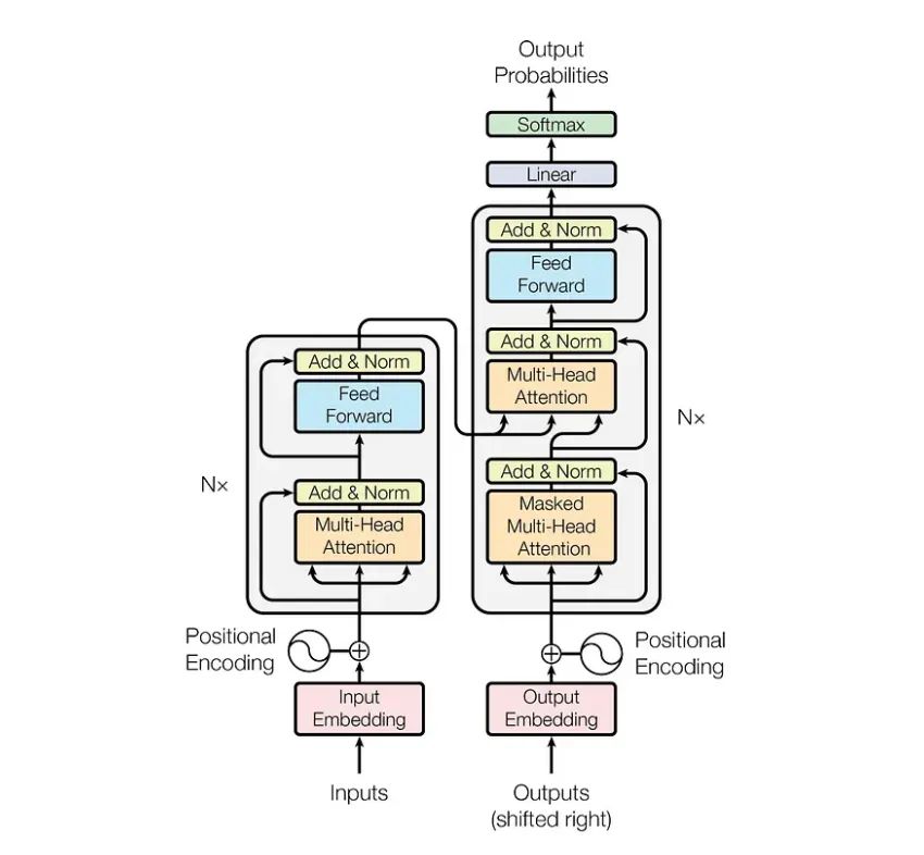
Model Architecture

LLM in Brief​

Many believe that large models can directly answer questions or engage in conversations. However, their core function is to predict the next likely word, or "Token," based on the input text. This predictive ability makes LLMs excel in various applications, including but not limited to:

  • Text Generation: LLMs can generate coherent and meaningful text passages for writing assistance, content creation, etc.
  • Question Answering Systems: By understanding the context of a question, LLMs can generate accurate answers, widely used in intelligent customer service and information retrieval.
  • Translation: LLMs can perform high-quality language translation based on context, supporting multilingual communication.
  • Text Summarization: LLMs can extract key content from long documents to generate concise summaries, facilitating quick understanding.
  • Dialogue Systems: LLMs can simulate human conversations, providing natural and smooth interaction experiences, applied in chatbots and virtual assistants.

By understanding the concept of Tokens, we can better grasp the working principles of LLMs and their powerful capabilities in practical applications.

Token​

Example​

When discussing Tokens, it's impossible not to mention a recent low-level error in a large model: "How many 'r's are in 'Strawberry'?"

Strawberry

After the ridicule, people calmed down and began to think: what is the essence behind this low-level error?

It is generally believed that it is the fault of Tokenization.

In China, Tokenization is often translated as "word segmentation." This translation is somewhat misleading because the Tokens in Tokenization do not necessarily refer to words; they can also be punctuation marks, numbers, or parts of a word. For example, in a tool provided by OpenAI, the word "Strawberry" is divided into three Tokens: Str-aw-berry. In this case, asking the AI large model to count how many 'r's are in the word is indeed a challenge for it.

To let everyone intuitively see the world of text in the eyes of large models, Karpathy specially wrote a small program to represent Tokens with emojis.
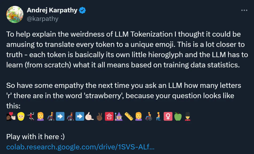
Tokens With Emojis

Attempt​

A Token is the basic unit of text that LLMs understand. Although it is convenient to consider a Token as a word, for LLMs, the goal is to encode text as efficiently as possible. Therefore, in many cases, a Token represents a character sequence shorter or longer than an entire word. Punctuation marks and spaces are also represented as Tokens, either individually or combined with other characters. Each Token in the LLM vocabulary has a unique identifier, usually a number. LLMs use tokenizers to convert regular text strings into equivalent lists of Token numbers.

import tiktoken

# Get the encoder for the GPT-2 model
encoding = tiktoken.encoding_for_model("gpt-2")

# Encode example sentence
encoded_text = encoding.encode("A journey of a thousand miles begins with a single step.")
print(encoded_text)

# Decode back to original text
decoded_text = encoding.decode(encoded_text)
print(decoded_text)

# Encode and decode individual tokens
print(encoding.decode([32])) # 'A'
print(encoding.decode([7002])) # ' journey'
print(encoding.decode([286])) # 'of'

# Encode the word "thousand"
thousand_encoded = encoding.encode("thousand")
print(thousand_encoded)

# Decode the encoded result of "thousand"
print(encoding.decode([400])) # 'th'
print(encoding.decode([29910])) # 'ousand'

[32, 7002, 286, 257, 7319, 4608, 6140, 351, 257, 2060, 2239, 13]
A journey of a thousand miles begins with a single step.
A
journey
of
[400, 29910]
th
ousand

Predicting the Next Token​

As mentioned above, given a piece of text, the task of a language model is to predict the next Token. If expressed in Python pseudocode, it looks like this:

predictions = predict_next_token(['A', 'journey', 'of', 'a'])

Here, the predict_next_token function receives a series of input Tokens converted from a user-provided prompt. In this example, we assume each word constitutes a separate Token. In reality, each Token is encoded as a number rather than being directly passed into the model as text. The output of the function is a data structure containing the probability values for each possible Token in the vocabulary to appear after the current input sequence.

The language model needs to learn to make such predictions through a training process. During training, the model is exposed to a large amount of text data, learning language patterns and rules. After training, the model can use the learned knowledge to estimate the probability of the next Token for any given Token sequence.

To generate continuous text, the model needs to repeatedly call itself, generating a new Token each time and adding it to the existing sequence until the preset length is reached. Below is a more detailed Python pseudocode showing this process:

def generate_text(prompt, num_tokens, hyperparameters):
tokens = tokenize(prompt) # Convert prompt to a list of Tokens
for _ in range(num_tokens): # Repeat for the specified number of Tokens
predictions = predict_next_token(tokens) # Get predictions for the next Token
next_token = select_next_token(predictions, hyperparameters) # Select the next Token based on probabilities
tokens.append(next_token) # Add the selected Token to the list
return ''.join(tokens) # Merge the Token list into a string

# Helper function to select the next Token
def select_next_token(predictions, hyperparameters):
# Adjust Token selection using strategies like temperature, top-k, or top-p
# Implementation details depend on the specific hyperparameter settings
pass

In this code, the generate_text function accepts a prompt string, the number of Tokens to generate, and a set of hyperparameters as input. The tokenize function is responsible for converting the prompt into a list of Tokens, while the select_next_token function selects the next Token based on the predicted probability distribution. By adjusting the hyperparameters in select_next_token, such as temperature, top-k, and top-p, the diversity and creativity of the generated text can be controlled. As the loop iterates, new Tokens are continuously added to the sequence, eventually forming coherent text output.

Model Training​

Imagine we are training a model to predict the next word in a sentence. This is like playing a word-guessing game where the model needs to guess the next word based on the words already present. For a simplified vocabulary, let's assume there are only five words:

['I', 'you', 'love', 'oranges', 'grapes']

We do not consider spaces and punctuation, focusing only on these words.

We have three sentences as training data:

  • I love oranges
  • I love grapes
  • you love oranges

We can imagine a 5x5 table where each cell represents the number of times one word follows another. This table might look like this:
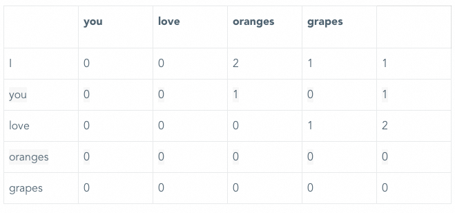
Cell Matrix

In this example, "I" is followed by "love" twice, and "love" is followed by "oranges" once and "grapes" twice. To make this table useful, we need to convert these counts into probabilities so that the model can predict the likelihood of the next word. For example, the probability of "oranges" following "love" is 1/3 (about 33.3%), and the probability of "grapes" following "love" is 2/3 (about 66.7%).

However, we encounter a problem: "oranges" and "grapes" do not appear after other words. This means that without additional information, the model will not be able to predict what might follow these words. To solve this problem, we can assume that any word in the vocabulary might follow any other word, although this is not perfect, it ensures that the model can make predictions even with limited training data.

In the real world, large language models (LLMs) use vast amounts of training data, reducing the chances of such "gaps" occurring. However, due to the infrequent occurrence of certain word combinations in the training data, LLMs may perform poorly in some cases, resulting in generated text that is grammatically correct but logically flawed or inconsistent. This phenomenon is sometimes referred to as "model hallucination."

Context Window​

In previous discussions, we mentioned using Markov chains to train small models, which rely on only the last Token to predict the next Token. This means that any text before the last Token does not affect the prediction, so the context window is very small, only one Token. Due to the small context window, the model easily "forgets" previous information, leading to generated text that lacks consistency, jumping from one word to another.

Improving the Context Window​

To improve the model's prediction quality, we can try to increase the size of the context window. For example, if we use a two-Token context window, we need to build a larger probability matrix where each row represents all possible two-Token sequences. For a five-Token vocabulary, this will add 25 rows (5^2). Each time the predict_next_token() function is called, the last two Tokens of the input will be used to find the corresponding row in the probability table.

However, even with a two-Token context window, the generated text may still lack coherence. To generate more consistent and meaningful text, the context window size needs to be further increased. For example, increasing the context window to three Tokens will increase the number of rows in the probability table to 125 (5^3), but this is still insufficient to generate high-quality text.

As the context window increases, the size of the probability table grows exponentially. Taking the GPT-2 model as an example, it uses a 1024-Token context window. If we were to implement such a large context window using Markov chains as in the previous example, each row of the probability table would need to represent a sequence of length between 1 and 1024 Tokens. For a vocabulary of 5 Tokens, the number of possible sequences is 5^1024, an astronomical number. This number is so large that it is impractical to store and process such a massive probability table. Therefore, Markov chains face serious scalability issues when dealing with large context windows.

From Markov Chains to Neural Networks​

Clearly, the probability table method is infeasible when dealing with large context windows. We need a more efficient method to predict the next Token. This is where neural networks come into play. Neural networks are special functions that accept input data, perform a series of calculations, and then output predictions. For language models, the input is a series of Tokens, and the output is the probability distribution of the next Token.

The key to neural networks lies in their parameters. These parameters are gradually adjusted during training to optimize the model's prediction performance. The training process involves extensive mathematical operations, including forward propagation and backpropagation. Forward propagation refers to the input data passing through the network's layers to generate predictions; backpropagation adjusts the network's parameters based on the difference between the predictions and the true labels to reduce errors.

Modern language models, such as GPT-2, GPT-3, and GPT-4, use very deep neural networks with hundreds of millions or even trillions of parameters. The training process for these models is very complex and usually takes weeks or even months. Despite this, well-trained LLMs maintain high coherence and consistency in text generation, thanks to their powerful context understanding and generation capabilities.

Transformer and Attention Mechanism​

The Transformer is one of the most popular neural network architectures, particularly suited for natural language processing tasks. The core feature of the Transformer model is its attention mechanism. The attention mechanism allows the model to dynamically focus on different parts of the input sequence when processing it, thereby better capturing context information.

The attention mechanism was initially applied to machine translation tasks to help the model identify key information in the input sequence. Through the attention mechanism, the model can "focus" on important Tokens in the input sequence, thereby generating more accurate translation results. In language generation tasks, the attention mechanism plays an equally important role, enabling the model to consider multiple Tokens in the context window when generating the next Token, thereby generating more coherent and meaningful text.

In summary, although Markov chains provide a simple method for text generation, they have obvious limitations when dealing with large context windows. Modern language models overcome these limitations by using neural networks and attention mechanisms, achieving efficient and high-quality text generation.
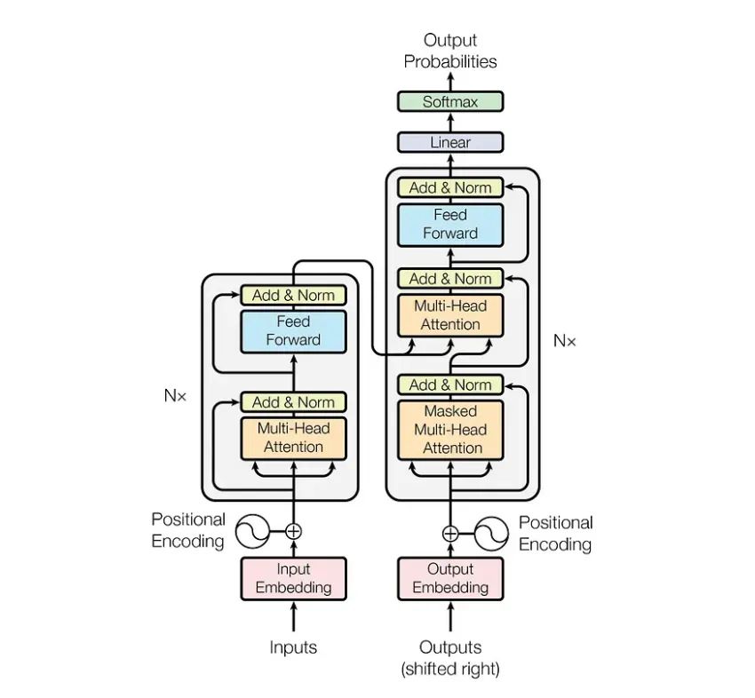
Framework-05

Returning to the framework diagram, the input representation x of a word in the Transformer is obtained by adding the word Embedding and the position Embedding (Positional Encoding).

There are many ways to obtain the word Embedding, such as using pre-trained algorithms like Word2Vec, Glove, or training it in the Transformer.

In addition to the word Embedding, the Transformer also uses position Embedding to represent the position of a word in the sentence. Because the Transformer does not use an RNN structure but uses global information, it cannot utilize the order information of words, which is very important for NLP. Therefore, the Transformer uses position Embedding to preserve the relative or absolute position of words in the sequence.

In short: taking "apple" as an example

In "There are apples and bananas in the fruit store," "apple" refers to the fruit, while in "The store has just launched the latest Apple 16," "apple" represents the brand.

Self-Attention (Self-Attention Mechanism)​

Self Attention

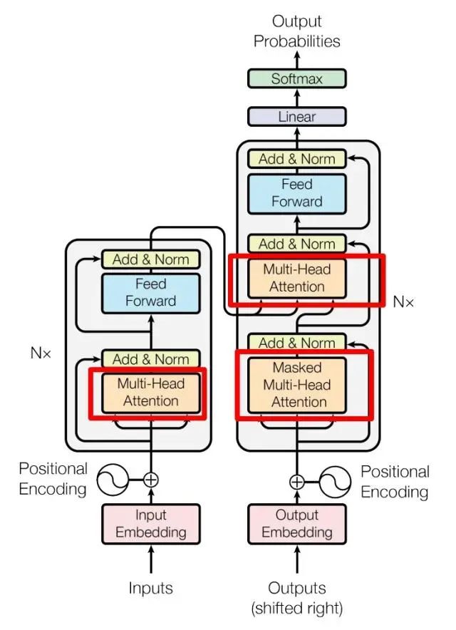
The above image is the internal structure diagram of the Transformer in the paper, with the left side being the Encoder block and the right side being the Decoder block. The part circled in red is Multi-Head Attention, which consists of multiple Self-Attention layers. It can be seen that the Encoder block contains one Multi-Head Attention, while the Decoder block contains two Multi-Head Attention (one of which uses Masked). Above the Multi-Head Attention is an Add & Norm layer, where Add represents a residual connection (Residual Connection) to prevent network degradation, and Norm represents Layer Normalization to normalize the activation values of each layer.

Since Self-Attention is the key point of the Transformer, we focus on Multi-Head Attention and Self-Attention. First, let's take a detailed look at the internal logic of Self-Attention.

Of course, we can understand the Self-Attention mechanism in a more concise way.

Self-Attention Introduction​

Self-Attention is a method that allows the model to focus on different parts of the sequence data when processing it, especially suitable for handling long texts. It achieves this by calculating the relevance between each element in the sequence and all other elements.

Workflow​

  1. Transformation:

    • Each input element (such as a word) is transformed into three vectors: Query (query), Key (key), and Value (value). These vectors are obtained by multiplying the input vector by three different weight matrices WQ, WK, and WV.
  2. Calculate Attention Scores:

    • For each element, use its Query vector to perform dot product operations with the Key vectors of all other elements, obtaining a list of scores. This score represents the relevance of the current element to all other elements.
  3. Normalization:

    • Normalize these scores through the softmax function to obtain a probability distribution, representing the attention weights of the current element to all other elements.
  4. Weighted Sum:

    • Use these attention weights to perform a weighted sum of the Value vectors of all elements, obtaining the final output vector.

Formula​

Suppose the input sequence is X = [x1, x2, ..., xn], where each xi is a vector.

  1. Transformation:

Transformation

  1. Calculate Attention Scores:

Calculate Attention

where dk is the dimension of the Key vector.

  1. Normalization: Attention Weights = softmax(Scores)

  2. Weighted Sum: Output = Attention Weights · V

Multi-Head Attention​

  • Multi-Head Attention is designed to allow the model to capture information from multiple different perspectives. Specifically, multiple Self-Attention layers (each called a "head") are run in parallel, and then all heads' outputs are concatenated and passed through a linear transformation.

Summary​

  • Self-Attention allows the model to focus on different parts of the sequence, thereby better capturing long-range dependencies.
  • Multi-Head Attention enhances the model's expressive power by using multiple Self-Attention layers, allowing it to consider information from multiple perspectives.

Add & Norm and Feed Forward​

Add & Norm (Residual Connection and Layer Normalization)​

Residual Connection​

  • Purpose: The residual connection helps in training deep networks by allowing the gradient to flow directly through the network, mitigating the vanishing gradient problem.
  • Operation: The residual connection adds the input of a layer directly to its output: [ \text{Output} = F(x) + x ] where ( F(x) ) is the output of the layer.

Layer Normalization​

  • Purpose: Layer normalization stabilizes the training process by normalizing the activations of each layer, ensuring that the mean and variance of the activations remain consistent.
  • Operation: For each sample in the batch, layer normalization normalizes the activations across the feature dimension: [ \text{LayerNorm}(x) = \frac{x - \mu}{\sigma} \cdot \gamma + \beta ] where ( \mu ) and ( \sigma ) are the mean and standard deviation of the activations, and ( \gamma ) and ( \beta ) are learnable parameters.

Combined Use​

  • Steps:

    1. First, calculate the output ( F(x) ) of a layer.
    2. Add the input ( x ) to ( F(x) ), obtaining ( y = F(x) + x ).
    3. Perform layer normalization on ( y ) to obtain the final output.

Feed Forward Neural Network​

Purpose​

  • Add Nonlinearity: Makes the model more flexible, capable of handling more complex data.

Structure​

  • Two-Layer Fully Connected Network:

    1. The first layer: Transform the input through a linear transformation (multiply by a matrix), then process it with the ReLU activation function.
    2. The second layer: Transform it again through a linear transformation (multiply by another matrix).

Summary​

  • Add & Norm: Through residual connections and layer normalization, the model becomes more stable and trains faster.
  • Feed Forward: Through a two-layer fully connected network, it adds flexibility to the model, enabling it to handle more complex data.

Decoder Structure​

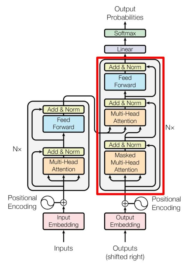
Decoder Structure

The red part in the above image is the structure of the Transformer's Decoder block, similar to the Encoder block but with some differences:

  • Contains two Multi-Head Attention layers.
  • The first Multi-Head Attention layer uses a Masked operation.
  • The second Multi-Head Attention layer's K, V matrices use the Encoder's encoded information matrix C for calculation, while Q uses the output of the previous Decoder block for calculation.
  • Finally, a Softmax layer calculates the probability of the next translated word.

Appendix​

# Import necessary libraries
import torch
import torch.nn as nn
import torch.optim as optim
import math

# Define the positional encoding layer, used to add positional information to the input sequence
class PositionalEncoding(nn.Module):
def __init__(self, d_model, max_len=5000):
super(PositionalEncoding, self).__init__()
# Initialize the positional encoding tensor
pe = torch.zeros(max_len, d_model)
position = torch.arange(0, max_len, dtype=torch.float).unsqueeze(1)
div_term = torch.exp(torch.arange(0, d_model, 2).float() * (-math.log(10000.0) / d_model))
# Calculate the sine and cosine values
pe[:, 0::2] = torch.sin(position * div_term)
pe[:, 1::2] = torch.cos(position * div_term)
pe = pe.unsqueeze(0).transpose(0, 1)
# Register the positional encoding as a buffer
self.register_buffer('pe', pe)

def forward(self, x):
# Add the positional encoding to the input
x = x + self.pe[:x.size(0), :]
return x

# Define the Transformer-based model class
class TransformerModel(nn.Module):
def __init__(self, input_dim, output_dim, d_model=512, nhead=8, num_encoder_layers=6, dim_feedforward=2048, dropout=0.1):
super(TransformerModel, self).__init__()
self.model_type = 'Transformer'
# Define the embedding layer
self.embedding = nn.Embedding(input_dim, d_model)
# Define the positional encoding layer
self.pos_encoder = PositionalEncoding(d_model)
# Define the encoder layers
encoder_layers = nn.TransformerEncoderLayer(d_model, nhead, dim_feedforward, dropout)
self.transformer_encoder = nn.TransformerEncoder(encoder_layers, num_encoder_layers)
self.d_model = d_model
# Define the decoder layer
self.decoder = nn.Linear(d_model, output_dim)
# Initialize the weights
self.init_weights()

def init_weights(self):
initrange = 0.1
self.embedding.weight.data.uniform_(-initrange, initrange)
self.decoder.bias.data.zero_()
self.decoder.weight.data.uniform_(-initrange, initrange)

def forward(self, src, src_mask):
# Embed the input and multiply by the square root of d_model
src = self.embedding(src) * math.sqrt(self.d_model)
src = self.pos_encoder(src)
# Encode the input
output = self.transformer_encoder(src, src_mask)
# Decode the output
output = self.decoder(output)
return output

# Generate a triangular matrix as a mask
def generate_square_subsequent_mask(sz):
mask = (torch.triu(torch.ones(sz, sz)) == 1).transpose(0, 1)
mask = mask.float().masked_fill(mask == 0, float('-inf')).masked_fill(mask == 1, float(0.0))
return mask

# Example usage
input_dim = 1000 # Vocabulary size
output_dim = 1000 # Output dimension
seq_length = 10 # Sequence length

# Create a model instance
model = TransformerModel(input_dim=input_dim, output_dim=output_dim)

# Example data
src = torch.randint(0, input_dim, (seq_length, 32)) # (sequence length, batch size)
src_mask = generate_square_subsequent_mask(seq_length)

# Forward propagation
output = model(src, src_mask)
print(output.shape) # Expected output: [sequence length, batch size, output dimension]

# Define a simple loss function and optimizer for training
criterion = nn.CrossEntropyLoss()
optimizer = optim.Adam(model.parameters(), lr=0.001)

# Example training loop
for epoch in range(10): # Number of iterations
optimizer.zero_grad()
output = model(src, src_mask)
loss = criterion(output.view(-1, output_dim), src.view(-1))
loss.backward()
optimizer.step()
print(f"Epoch {epoch+1}, Loss: {loss.item()}")